Basics GPU ML re-cap from 2025-02

Ref Learn GPU Programming with Youtube Simon Oz

Dates:

• [2025-02-26-Wednesday]
• [2025-02-27-Thursday]
• [2025-02-28-Friday]

这里我们还是先考虑单色 picture as input。这样的话我们目前可以先不考虑 Tensor 的问题，不涉及张量，input batch 只是一个 2D matrix.

About how to understand the dimensions

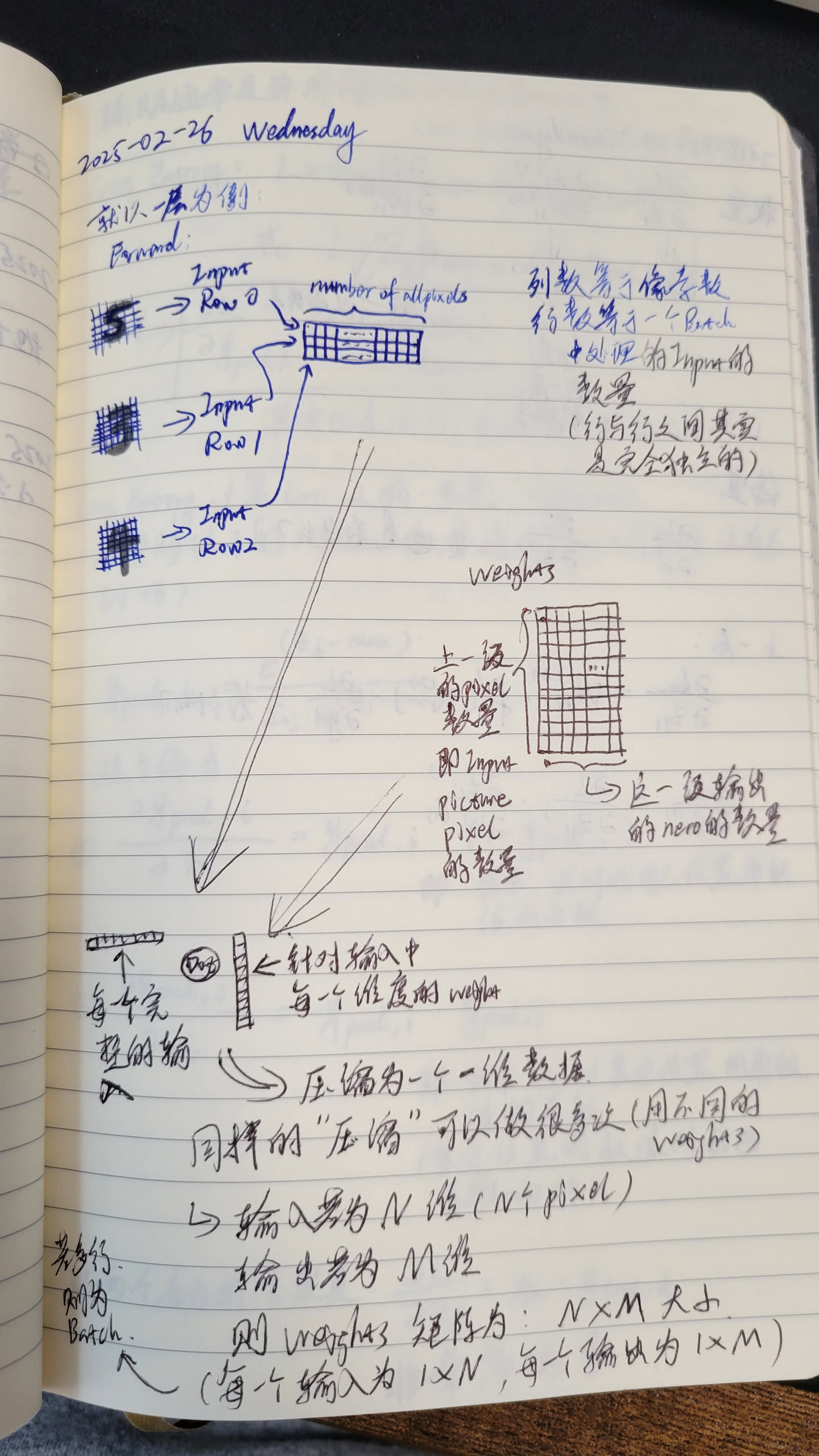
所以 对于第一层 weight 矩阵，仅仅是 num_rows = number_of_pixels_in_each_input_image, num_colums = dimensions_of_the_output_vector.

weights 矩阵的每一列，相当于对于整个 input 进行一次压缩，压缩为一个标量 (one pixel)。 多个列就是进行多次压缩，最终组合成一个新的向量。

Forward propagation

Weights

__global__ void forward(
  int batch_size, // this is also the number of rows for the input matrix,
                  // each row is one picture.
  int input_width, // this is the width of the input matrix, 
                   // i.e. the number of colums for the input matrix, 
                   // i.e. number of pixels in each input image
  int out_width, // output width, i.e. number of colums for weights matrix
  float* input, // the flatten input array
  float* biases, // the flatten bias array, this should be (1, out_width) shape
  float* output, // the flatten output array
) {
  // blockDim includes the number of 'threads' per block in each dimension
  // blockIdx is the index of 'block'.
  // Following is used to locate **one** element in the **output** matrix!
  // output matrix num_of_row is determined by the batch_size
  // output matrix num_of_colums is determined by the out_width (the weight matrix num_of_colums)
  // out_row_index must be less than batch_size
  // out_column_index must be less than out_width
  int out_column_index = blockIdx.x * blockDim.x + threadIdx.x;
  int out_row_index = blockIdx.y * blockDim.y + threadIdx.y;
 
  if (out_row_index < batch_size && out_column_index < out_width) {
    int output_elem = out_row_index * out_width + out_column_index;
    // Add the biases first.
    output[output_elem] = biases[out_column_index];
    // do the matrix multiplication for each output element
    for (int i = 0; i < input_width; i++) {
      int input_elem = out_row_index * input_width + i;
      int weights_elem = i * out_width + out_column_index;
      output[output_elem] += input[input_elem] * weights[weights_elem];
    }
  }
 
}

NOTE

$biases$ 实际上是一个行向量，只不过重复了 $batc{h}_{s}ize$ 次。看起来是个矩阵，但是其实只是行向量。

Activation

ReLU is used as the activation function for the hidden layers.

ReLU activation function:

$$ReLU(x)=\{\begin{array}{ll}x& \text{if x > 0}\\ 0& \text{if x <= 0}\end{array}$$

__global__ void relu(
  int batch_size, // this is also the number of rows for the input matrix,
                  // each row is one picture.
  int out_width, // output width, also number of columns for weights matrix 
                 // from the prior stage.
                 // for this ReLU, input and output have the same shape.
  float* input, // the flatten input array
  float* output, // the flatten output array
) {
  int out_column_index = blockIdx.x * blockDim.x + threadIdx.x;
  int out_row_index = blockIdx.y * blockDim.y + threadIdx.y;
 
  if (out_row_index < batch_size && out_column_index < out_width) {
    int out_index = out_row_index * out_width + out_column_index;
    float act = input[out_index];
    output[out_index] = act > 0.0f ? act : 0.f;
  }
}

Softmax

Softmax is used as the activation function for the last layer.

$$softmax(x_i)=\frac{e^{x_i-max(x)}}{{\sum }_{j=1}^n{e}^{x_j-max(x)}}$$

And $n$ is the number of colums.

__global__ void softmax(
  int batch_size, // this is also the number of rows for the input matrix,
  int out_width, // output width, also number of colums for weights matrix
                 // from the prior stage.
                 // for this softmax, input and output have the same shape.
  float* input, // the flatten input array
  float* output, // the flatten output array
) {
  int out_column_index = blockIdx.x * blockDim.x + threadIdx.x;
  int out_row_index = blockIdx.y * blockDim.y + threadIdx.y;
 
  if (out_row_index < batch_size && out_column_index < out_width) {
    // init the max with the first value in the row
    float max_val = input[out_row_index * out_width]; 
    for (int it = 1; it < out_width; it++) {
      max_val =  max(max_val, input[out_row_index * out_width + it]);
    }
    // calculate divisor
    float divisor = 0.f;
    for (int j = 0; j < out_width; j++) {
      divisor += exp(input[out_row_index * out_width + j] - max_val);
    }
    // final dividing
    int out_index = out_row_index * out_width + out_column_index;
    output[output_index] = exp(input[out_index] - max_val) / divisor;
  }
}

Loss function

$$L=-\sum _{i=1}^n{p}_i\log q_i$$

$p_i$ is the true label, $q_i$ is the predicted label.

对于一个 input (就是 batch 中的一行)，$L$是一个标量。

__global__ void cross_entropy(
  int batch_size, // this is also the number of rows for the input matrix,
  int input_width, // this is the width of the input matrix,
  float* pred, // the flatten input array, predicated label
  float* actual, // the flatten actual array, shape: (batch_size, input_width),
                 // only one column per row is 1.0, others are 0.0
  float* loss, // the flatten loss array, shape: (batch_size, 1)
) {
  int out_row_index = blockIdx.y * blockDim.y + threadIdx.y;
  if (out_row_index < batch_size) {
    float loss_val = 0.f;
    // iterate through each column per for the current row
    for (int i = 0; i < input_width; i++) {
      int curr_idx = out_row_index * input_width + i;
      // use ie-6 to avoid log(0)
      loss -= actual[curr_idx] * log(max(ie-6, pred[curr_idx]));
    }
  }
}

First stop of Backpropagation

For the very last layer, the partial derivative of the loss function to the raw output (not the output after softmax) is:

For one input (i.e. one row):

$$\frac{\partial L}{\partial x_i}=s_i-y_{real,i}$$

$s_i$ is the ‘softmax’ result of the last layer at $i$ column

$y_{real,i}$ is the true label value at $i$ column

$i$ is the index in one row (one row represents one original input data: i.e. picture)

And each row is basically independent, so we still can batch them together.

详细推导过程 [detailed-derivation-partial-derivative-of-the-loss-value-to-the-last-layer-raw-output]

__global__ void cross_entropy_backprop(
  int batch_size, // this is also the number of rows for the input matrix,
  int preds_width, // the width of the 'preds' and 'actual' matrix
  float* preds, // the flatten input array, predicated label
  float* actual, // the flatten actual array, shape: (batch_size, preds_width),
  float* output, // the partial derivative of the raw output of the last layer
                 // the shape is (batch_size, preds_width). Note that this is 
                 // not the 'weights' matrix shape. The shape of the last layer
                 // weights matrix should be:
                 // - Rows: last layer input data width,
                 // - Columns: preds_wdith (or actual_wdith).
) {
  int in_column_index = blockIdx.x * blockDim.x + threadIdx.x;
  int in_row_index = blockIdx.y * blockDim.y + threadIdx.y;
  if (in_row_index < batch_size && in_column_index < preds_width) {
    int idx =  in_row_index * preds_width + in_column_index;
    output[idx] = preds[idx] - actual[idx];
  }
}

Note the shape of the output matrix: (batch_size, preds_width) is very different from the shape of the weights matrix: (last_layer_input_data_width, preds_width), which is also: (prior_layer_weight_columns, preds_width).

所以其实每一个 weight matrix 的形状都是：(prior_layer_weight_columns, this_layer_weight_columns) = (prior_layer_weight_columns, this_layer_output_data_width).

再说一次，这里计算的实际上是

$$\frac{\partial L}{\partial X}$$

这里 $X$ 是 最后一层的 raw output, 纬度是 (batch_size, preds_width). 这个 $pred{s}_{w}idth$ 实际上也跟最后的 actual label width 是相同的。$X$ 虽然是一个矩阵，但是其实每一行都是独立的一个 input, 所以其本质是一个行向量。然后摆在一起，算是一个矩阵。

另外，这里 $L$ 实际上是对每个 row 有一个单独的值。所以是一个列向量。但是实际上 $L$ 针对每一个 input，可以看作一个标量。input 之间（不同行之间）实际上是独立的，所以本质是一个标量，摆在一起算是一个列向量。

这里面其实是还有个问题。就是这个 $\frac{\partial L}{\partial W}$ 的纬度问题。

关于 $\frac{\partial L}{\partial W}$ 的 shape 以及计算

先说结论：

• 最终 $\frac{\partial L}{\partial W}$ 的 shape 是：(prior_layer_weight_columns, this_layer_weight_columns), 即：(prior_layer_weight_columns, this_layer_output_data_width), 即：(prior_layer_weight_columns, $X$向量的宽度)。

• $\frac{\partial L}{\partial W}$ 的计算是：

$$\frac{\partial L}{\partial W}=a^T\cdot \frac{\partial L}{\partial X}$$

其中 $a$ 是上次层经过 activation 之后的输出。

l另外，这里面还必须要用到 transtive rule, (至少对于标量，有交换律，所以这个是完全成立的): $\frac{\partial L}{\partial X}=\frac{\partial L}{\partial Z}\cdot \frac{\partial Z}{\partial X}$

然后我们开始推导：我们首先假设我们只关注 input 1 这一行的 输入

$$\begin{gathered} X_{input1}=\left[\begin{array}{ccc}{x}_{input1,1}& x_{input1,2}& x_{input1,3}\end{array}\right] \\ = \\ \left[\begin{array}{ccc}{a}_{input1,1}{w}_{1,1}+a_{input1,2}{w}_{2,1}+a_{input1,3}{w}_{3,1}+b_1& a_{input1,1}{w}_{1,2}+a_{input1,2}{w}_{2,2}+a_{input1,3}{w}_{3,2}+b_2& a_{input1,1}{w}_{1,3}+a_{input1,2}{w}_{2,3}+a_{input1,3}{w}_{3,3}+b_3\end{array}\right] \\ = \\ {a}_{input1}\cdot W^n \end{gathered}$$

其中 $a_{input1}$ 是 input1 上一层，经过 activation 之后的输出。其中 $W^n$ 是第 N 层的权重矩阵。

NOTE

注意这里采用的是 $Z=AW$ 的计算方式，实际上在学术届，一般是 $Z=WA$ 的形式，就是说 W 对 A 这个 n 维向量做线性变换到 Z 这个 m 维向量。而 Z 和 A 都是列向量。

但是工业界一般是把 Z 和 A 用行向量表示，于是从学术的表示就变成 $Z^T=A^T{W}^T$。所以工业界的这个权重矩阵很可能跟学术届的表示是转置的关系。

所以：

$$\begin{gathered} \frac{\partial L_{input1}}{\partial W}=\left[\begin{array}{ccc}\frac{\partial L_{input1}}{\partial W_{1,1}}& \frac{\partial L_{input1}}{\partial W_{1,2}}& \frac{\partial L_{input1}}{\partial W_{1,3}}\\ \frac{\partial L_{input1}}{\partial W_{2,1}}& \frac{\partial L_{input1}}{\partial W_{2,2}}& \frac{\partial L_{input1}}{\partial W_{2,3}}\\ \frac{\partial L_{input1}}{\partial W_{3,1}}& \frac{\partial L_{input1}}{\partial W_{3,2}}& \frac{\partial L_{input1}}{\partial W_{3,3}}\end{array}\right]=\left[\begin{array}{ccc}\frac{\partial L_{input1}}{\partial X_{input1,1}}\cdot a_{input1,1}& \frac{\partial L_{input1}}{\partial X_{input1,2}}\cdot a_{input1,1}& \frac{\partial L_{input1}}{\partial X_{input1,3}}\cdot a_{input1,1}\\ \frac{\partial L_{input1}}{\partial X_{input1,1}}\cdot a_{input1,2}& \frac{\partial L_{input1}}{\partial X_{input1,2}}\cdot a_{input1,2}& \frac{\partial L_{input1}}{\partial X_{input1,3}}\cdot a_{input1,2}\\ \frac{\partial L_{input1}}{\partial X_{input1,1}}\cdot a_{input1,3}& \frac{\partial L_{input1}}{\partial X_{input1,2}}\cdot a_{input1,3}& \frac{\partial L_{input1}}{\partial X_{input1,3}}\cdot a_{input1,3}\end{array}\right] \\ = \\ \left[\begin{array}{c}{a}_{input1,1}\\ a_{input1,2}\\ a_{input1,3}\end{array}\right]\cdot \left[\begin{array}{ccc}\frac{\partial L_{input1}}{\partial X_{input1,1}}& \frac{\partial L_{input1}}{\partial X_{input1,2}}& \frac{\partial L_{input1}}{\partial X_{input1,3}}\end{array}\right] \\ = \\ {a}_{input1}^T\cdot \frac{\partial L_{input1}}{\partial X_{input1}} \end{gathered}$$

之后再考虑多个 input 的情况，也就是 $X$ 纵向扩展（行扩展），然后 $a^T$ 横向扩展（列扩展）。这些扩展出来的都是对应的，然后会 sum 到一起。

$$\begin{gathered} \frac{\partial L_{input1}}{\partial W}+\frac{\partial L_{input2}}{\partial W} \\ = \\ \left[\begin{array}{ccc}\frac{\partial L_{input1}}{\partial W_{1,1}}& \frac{\partial L_{input1}}{\partial W_{1,2}}& \frac{\partial L_{input1}}{\partial W_{1,3}}\\ \frac{\partial L_{input1}}{\partial W_{2,1}}& \frac{\partial L_{input1}}{\partial W_{2,2}}& \frac{\partial L_{input1}}{\partial W_{2,3}}\\ \frac{\partial L_{input1}}{\partial W_{3,1}}& \frac{\partial L_{input1}}{\partial W_{3,2}}& \frac{\partial L_{input1}}{\partial W_{3,3}}\end{array}\right]+\left[\begin{array}{ccc}\frac{\partial L_{input2}}{\partial W_{1,1}}& \frac{\partial L_{input2}}{\partial W_{1,2}}& \frac{\partial L_{input2}}{\partial W_{1,3}}\\ \frac{\partial L_{input2}}{\partial W_{2,1}}& \frac{\partial L_{input2}}{\partial W_{2,2}}& \frac{\partial L_{input2}}{\partial W_{2,3}}\\ \frac{\partial L_{input2}}{\partial W_{3,1}}& \frac{\partial L_{input2}}{\partial W_{3,2}}& \frac{\partial L_{input2}}{\partial W_{3,3}}\end{array}\right] \\ = \\ \left[\begin{array}{ccc}\frac{\partial L_{input1}}{\partial x_{input1,1}}\cdot a_{input1,1}+\frac{\partial L_{input2}}{\partial x_{input2,1}}\cdot a_{input2,1}& \frac{\partial L_{input1}}{\partial x_{input1,2}}\cdot a_{input1,1}+\frac{\partial L_{input2}}{\partial x_{input2,2}}\cdot a_{input2,1}& \frac{\partial L_{input1}}{\partial x_{input1,3}}\cdot a_{input1,1}+\frac{\partial L_{input2}}{\partial x_{input2,3}}\cdot a_{input2,1}\\ \frac{\partial L_{input1}}{\partial x_{input1,1}}\cdot a_{input1,2}+\frac{\partial L_{input2}}{\partial x_{input2,1}}\cdot a_{input2,2}& \frac{\partial L_{input1}}{\partial x_{input1,2}}\cdot a_{input1,2}+\frac{\partial L_{input2}}{\partial x_{input2,2}}\cdot a_{input2,2}& \frac{\partial L_{input1}}{\partial x_{input1,3}}\cdot a_{input1,2}+\frac{\partial L_{input2}}{\partial x_{input2,3}}\cdot a_{input2,2}\\ \frac{\partial L_{input1}}{\partial x_{input1,1}}\cdot a_{input1,3}+\frac{\partial L_{input2}}{\partial x_{input2,1}}\cdot a_{input2,3}& \frac{\partial L_{input1}}{\partial x_{input1,2}}\cdot a_{input1,3}+\frac{\partial L_{input2}}{\partial x_{input2,2}}\cdot a_{input2,3}& \frac{\partial L_{input1}}{\partial x_{input1,3}}\cdot a_{input1,3}+\frac{\partial L_{input2}}{\partial x_{input2,3}}\cdot a_{input2,3}\end{array}\right] \\ = \\ \left[\begin{array}{cc}{a}_{input1,1}& a_{input2,1}\\ a_{input1,2}& a_{input2,2}\\ a_{input1,3}& a_{input2,3}\end{array}\right]\cdot \left[\begin{array}{ccc}\frac{\partial L_{input1}}{\partial x_{input1,1}}& \frac{\partial L_{input1}}{\partial x_{input1,2}}& \frac{\partial L_{input1}}{\partial x_{input1,3}}\\ \frac{\partial L_{input2}}{\partial x_{input2,1}}& \frac{\partial L_{input2}}{\partial x_{input2,2}}& \frac{\partial L_{input2}}{\partial x_{input2,3}}\end{array}\right] \\ = \\ {a}^T\cdot \frac{\partial L}{\partial X} \end{gathered}$$

所以这用 $a^T\cdot \frac{\partial L}{\partial X}$ 得到到结果是：batch里面所有input row最终的结果到 W 的偏导数的 合。

So, when updating the values in $W$, we need to take into account the batch_size. With a η as the learning rate, we should update the values in in $W$ by:

$$w(new)=w(old)-\frac{\eta }{batchSize}\cdot a^T\cdot \frac{\partial L}{\partial x}$$

注意，到目前为止，这里还只是针对最后一层

接下来推 $\frac{\partial L}{\partial biases}$

$$\begin{gathered} X_{input1}=\left[\begin{array}{ccc}{x}_{input1,1}& x_{input1,2}& x_{input1,3}\end{array}\right] \\ = \\ \left[\begin{array}{ccc}{a}_{input1,1}{w}_{1,1}+a_{input1,2}{w}_{2,1}+a_{input1,3}{w}_{3,1}+b_1& a_{input1,1}{w}_{1,2}+a_{input1,2}{w}_{2,2}+a_{input1,3}{w}_{3,2}+b_2& a_{input1,1}{w}_{1,3}+a_{input1,2}{w}_{2,3}+a_{input1,3}{w}_{3,3}+b_3\end{array}\right] \\ = \\ {a}_{input1}\cdot W^n \end{gathered}$$

所以

$$\left[\begin{array}{ccc}\frac{\partial L_{input1}}{\partial b_1}& \frac{\partial L_{input1}}{\partial b_2}& \frac{\partial L_{input1}}{\partial b_3}\end{array}\right]=\left[\begin{array}{ccc}\frac{\partial L_{input1}}{\partial x_{input1,1}}& \frac{\partial L_{input1}}{\partial x_{input1,2}}& \frac{\partial L_{input1}}{\partial x_{input1,3}}\end{array}\right]$$

然后我们把 1 个input 拓展到多个 input (i.e. batch_size != 1)

$$\left[\begin{array}{ccc}\frac{\partial L_{input1}}{\partial b_1}& \frac{\partial L_{input1}}{\partial b_2}& \frac{\partial L_{input1}}{\partial b_3}\\ \frac{\partial L_{input2}}{\partial b_1}& \frac{\partial L_{input2}}{\partial b_2}& \frac{\partial L_{input2}}{\partial b_3}\end{array}\right]=\left[\begin{array}{ccc}\frac{\partial L_{input1}}{\partial x_{input1,1}}& \frac{\partial L_{input1}}{\partial x_{input1,2}}& \frac{\partial L_{input1}}{\partial x_{input1,3}}\\ \frac{\partial L_{input2}}{\partial x_{input2,1}}& \frac{\partial L_{input2}}{\partial x_{input2,2}}& \frac{\partial L_{input2}}{\partial x_{input2,3}}\end{array}\right]$$

所以可以看出来，针对 $b$ 的偏导数，此时还没有 aggregated （not sumed yet)。每个 input 的 偏导数都是分开在每一行的。 那么针对一个 batch，我们还是要 sum 一下的。那这个就相当于纵向 sum，也可以理解成左乘一个 1 的行向量。

$$\begin{gathered} \left[\begin{array}{ccc}\frac{\partial L_{batch}}{\partial b_1}& \frac{\partial L_{batch}}{\partial b_2}& \frac{\partial L_{batch}}{\partial b_3}\end{array}\right]=\left[\begin{array}{ccc}\frac{\partial L_{input1}}{\partial b_1}+\frac{\partial L_{input2}}{\partial b_1}& \frac{\partial L_{input1}}{\partial b_2}+\frac{\partial L_{input2}}{\partial b_2}& \frac{\partial L_{input1}}{\partial b_3}+\frac{\partial L_{input2}}{\partial b_3}\end{array}\right] \\ = \\ \left[\begin{array}{ccc}\frac{\partial L_{input1}}{\partial x_{input1,1}}+\frac{\partial L_{input2}}{\partial x_{input2,1}}& \frac{\partial L_{input1}}{\partial b_2}+\frac{\partial L_{input2}}{\partial b_2}& \frac{\partial L_{input1}}{\partial b_3}+\frac{\partial L_{input2}}{\partial b_3}\end{array}\right] \\ = \\ \left[\begin{array}{cc}1& 1\end{array}\right]\cdot \left[\begin{array}{ccc}\frac{\partial L_{input1}}{\partial b_1}& \frac{\partial L_{input1}}{\partial b_2}& \frac{\partial L_{input1}}{\partial b_3}\\ \frac{\partial L_{input2}}{\partial b_1}& \frac{\partial L_{input2}}{\partial b_2}& \frac{\partial L_{input2}}{\partial b_3}\end{array}\right] \end{gathered}$$

所以：

$$\frac{\partial L}{\partial b}={\left[\begin{array}{c}1\\ 1\\ ...\\ 1\end{array}\right]}^T\cdot \frac{\partial L}{\partial X}$$

其实这个公式跟 $w$ 的公式是非常一致的。左乘的这个矩阵，宽度一样是 batch_size, 高度是 “1”，

• 只不过，对于 $w$, 左乘的这个矩阵的高度是上一个layer wegiths 的宽度，也就是 $a^{n-1}$ 的宽度.

故，学习的公式应该是：

$$b(new)=b(old)-\frac{\eta }{batchSize}\cdot [1,...,1]\cdot \frac{\partial L}{\partial x}$$

其中 [1, …, 1] 的宽度是 batch_size, 高度是 1.

w matrix and b vector update formula

$$w(new)=w(old)-\frac{\eta }{batchSize}\cdot a^T\cdot \frac{\partial L}{\partial x}$$ $$b(new)=b(old)-\frac{\eta }{batchSize}\cdot [1,...,1]\cdot \frac{\partial L}{\partial x}$$

So the code to update the last layer weights and biases together

__global__ void update_last_layer_weights(
  int w, int h,   // The width and height of the weights matrix
                  // the 'w' is also the width of the output of the last layer, i.e. width of 'x'
                  // the 'h' is also the width of the previous layer's output, i.e. width of 'a'
                  // 'h' is also the width of the previous layer's weights matrix.
  int batch_size, // The batch size.
  float lr,       // Learning rate.
  float* weights, // The weights matrix of the last layer.
  float* biases,  // The biases vector of the last layer, shape: [1 x w].
  float* a,       // The activation results of the previous layer, shape: [batch_size x h].
  float* dl_dx,   // The partial derivative of the loss function with respect to
                  // the raw output of the last layer, shape: [batch_size x w].
) {
  // row/col index means the location of in the weights matrix.
  // column index also represents the location in the biases row vector too.
  int col_index = blockIdx.x * blockDim.x + threadIdx.x;
  int row_index = blockIdx.y * blockDim.y + threadIdx.y;
 
  if (row_index >= h || col_index >= w) {
    return;
  }
 
  // calculate the a^T * dl_dx:
  // Full row of a^T with row_index -> Full column of a with row_index as column index,
  // Full column of dl_dx with col_index.
  float dw_sum = 0.0f;
  for (int i = 0; i < batch_size; i++) {
    dw_sum += a[i * h + row_index] * dl_dx[i * w + col_index];
  }
  // update weights
  weights[row_index * w + col_index] -= lr * dw_sum / float(batch_size); 
 
  // calculate the [1...1] * dl_dx:
  float db_sum = 0.0f;
  for (int i = 0; i < batch_size; i++) {
    db_sum += dl_dx[i * w + col_index];
  }
  // update biases
  biases[col_index] -= lr * db_sum / float(batch_size);
 
  // Notes for the biases update:
  // I think there are 'duplicated'  calculations here, because the biases updates
  // only needs to be calculated once. But the 'row_index' means this kernel will
  // be called multiple times in parallel.
  // But I guess this is fine for the correctness, because the 'duplicated'
  // caculations won't occur sequentially, but simultaneously and the read value
  // of biases[col_index] should all be the same for all kernel parallel threads.
  // So the final value written to the biases[col_index] in all parallel threads
  // will be exactly the same.
 
}

Backpropagation cross the weight matrix (i.e. weights output to weights input)

就是从第 N 层的 $x^n$ 的 $\frac{\partial L}{\partial x^n}$ 开始，算出来 针对第 N 层的输入，也就是上一层过了 activation 的输出 $a^{n-1}$ 的 $\frac{\partial L}{\partial a^{n-1}}$ 矩阵。

这里肯定就要用 $w^n$ 了。

先说一下公式：

$$\begin{gathered} X_{input1}=\left[\begin{array}{cc}{x}_{input1,1}& x_{input1,2}\end{array}\right] \\ = \\ \left[\begin{array}{cc}{a}_{input1,1}{w}_{1,1}+a_{input1,2}{w}_{2,1}+a_{input1,3}{w}_{3,1}+b_1& a_{input1,1}{w}_{1,2}+a_{input1,2}{w}_{2,2}+a_{input1,3}{w}_{3,2}+b_2\end{array}\right] \end{gathered}$$

So

$$\begin{gathered} \left[\begin{array}{ccc}\frac{\partial L_{input1}}{\partial a_{input1,1}}& \frac{\partial L_{input1}}{\partial a_{input1,2}}& \frac{\partial L_{input1}}{\partial a_{input1,3}}\end{array}\right] \\ = \\ \left[\begin{array}{ccc}\frac{\partial L_{input1}}{\partial x_{input1,1}}\frac{\partial x_{input1,1}}{\partial a_{input1,1}}+\frac{\partial L_{input1}}{\partial x_{input1,2}}\frac{\partial x_{input1,2}}{\partial a_{input1,1}}& \frac{\partial L_{input1}}{\partial x_{input1,1}}\frac{\partial x_{input1,1}}{\partial a_{input1,2}}+\frac{\partial L_{input1}}{\partial x_{input1,2}}\frac{\partial x_{input1,2}}{\partial a_{input1,2}}& \frac{\partial L_{input1}}{\partial x_{input1,1}}\frac{\partial x_{input1,1}}{\partial a_{input1,3}}+\frac{\partial L_{input1}}{\partial x_{input1,2}}\frac{\partial x_{input1,2}}{\partial a_{input1,3}}\end{array}\right] \\ = \\ \left[\begin{array}{ccc}\frac{\partial L_{input1}}{\partial x_{input1,1}}{w}_{1,1}+\frac{\partial L_{input1}}{\partial x_{input1,2}}{w}_{1,2}& \frac{\partial L_{input1}}{\partial x_{input1,1}}{w}_{2,1}+\frac{\partial L_{input1}}{\partial x_{input1,2}}{w}_{2,2}& \frac{\partial L_{input1}}{\partial x_{input1,1}}{w}_{3,1}+\frac{\partial L_{input1}}{\partial x_{input1,2}}{w}_{3,2}\end{array}\right] \\ = \\ \left[\begin{array}{cc}\frac{\partial L_{input1}}{\partial x_{input1,1}}& \frac{\partial L_{input1}}{\partial x_{input1,2}}\end{array}\right]\cdot \left[\begin{array}{ccc}{w}_{1,1}& w_{2,1}& w_{3,1}\\ w_{1,2}& w_{2,2}& w_{3,2}\end{array}\right] \\ = \\ \frac{\partial L_{input1}}{\partial x_{input1}}\cdot W^T \end{gathered}$$

然后拓展一下 batch_size，也就是 $\frac{\partial L}{\partial x}$ 变成多行的。 这个时候就会发现，最后结果还是 batch 中每一个 input 之间隔离的。就是说，batch 中某一行的 x 行向量 只参与了同一行的 $\frac{\partial L}{\partial x}$ 的计算, 计算出来的还是同一行的上一层的 $\frac{\partial L}{\partial a}$ 行向量。非常规整。这里并没有出现j计算$\frac{\partial L}{\partial w}$ 时出现的 sum 的情况。因为本质上 $a$ and $x$ 只是行向量。

$$\frac{\partial L}{\partial a^{n-1}}=\frac{\partial L}{\partial x^n}\cdot W^T$$

__global__ void backprop_layer(
  int batch_size,   // The batch size.
  int x_width,      // The width of the output of the layer, i.e. width of 'x'
  int a_width,      // The width of the input of the layer, i.e. width of 'a'
                    // This is also the heights of the current weights matrix.
  float* weights,   // The weights matrix of the layer, shape: [a_width x x_width].
  float* dl_dx,     // The partial derivative of the loss function with respect to
                    // the raw output of the layer, shape: [batch_size x x_width].
  float* dl_da,     // The partial derivative of the loss function with respect to
                    // the activation results of the previous layer, shape: [batch_size x a_width].
) {
  // now the index represents location in the dl_da matrix
  int col_index = blockIdx.x * blockDim.x + threadIdx.x;
  int row_index = blockIdx.y * blockDim.y + threadIdx.y;
 
  if (row_index >= batch_size || col_index >= a_width) {
    return;
  }
  float dl = 0.0f;
  for (int i = 0; i < x_width; i++) {
    // The Transformation for weights and weights_T:
    //  weights_T[i, j] = weights[j, i] = weights[j * x_width + i]
    dl += dl_dx[row_index * x_width + i] * weights[col_index * x_width + i];
  }
  dl_da[row_index * a_width + col_index] = dl;
}

ReLU 的 back propagation

因为中间 hidden layer 的 activation function is: $ReLU(x)=max(0,x)$, 所以 首先看看 ReLU 这一步， $a$ 是 ReLU 之后的结果， $x$ 是ReLU 的输入:

$$\left[\begin{array}{ccc}{a}_{input1,1}^n& a_{input1,2}^n& a_{input1,3}^n\end{array}\right]=\left[\begin{array}{ccc}max(0,x_{input1,1}^n)& max(0,x_{input1,2}^n)& max(0,x_{input1,3}^n)\end{array}\right]$$

NOTE

注意，这里的 ReLU 输入和输出都是同一层的。$x^n$ 经过 ReLU 之后就是 $a^n$。

这里因为ReLU其实不涉及矩阵乘法，所以我们直接针对每一个 $\frac{\partial L}{\partial x}$ 和 $\frac{\partial L}{\partial a}$ 的 matrix element 进行计算。

不过我们还是假定先搞定：input1 这一行。

$$\frac{\partial L_{input1}}{\partial x_{input1,i}}=\frac{\partial L_{input1}}{\partial a_{input1,i}}\cdot \frac{\partial a_{input1,i}}{\partial x_{input1,i}}=\{\begin{array}{ll}\frac{\partial L_{input1}}{\partial a_{input1,i}}& \text{if }{x}_{input1,i}>0\\ 0& \text{if }{x}_{input1,i}<=0\end{array}=\{\begin{array}{ll}\frac{\partial L_{input1}}{\partial a_{input1,i}}& \text{if }{a}_{input1,i}>0\\ 0& \text{if }{a}_{input1,i}=0\end{array}$$

Code below assumes we use $a_i$ instead of $x_i$ for branching.

__global__ void backprop_relu(
  int batch_size, // The batch size.
  int x_width,    // The width of the raw output of the layer, i.e. width of 'x'
                  // This is also the width of the weights matrix of this layer,
                  // though weights matrix is not used at all in this step.
  float* a        // The activation results of this layer, shape:
                  // [batch_size x x_width].
  float* dl_da    // The partial derivative of the loss function with respect to
                  // the activation results of this layer, shape:
                  // [batch_size x x_width].
  float* dl_dx    // The partial derivative of the loss function with respect to
                  // the raw output of this layer, shape:[batch_size x x_width].
) {
  int col_index = blockIdx.x * blockDim.x + threadIdx.x;
  int row_index = blockIdx.y * blockDim.y + threadIdx.y;
  if (row_index >= batch_size || col_index >= x_width) {
    return
  }
  float act_val = a[row_index * x_width + col_index];
  dl_dx[row_index * x_width + col_index] = act_val > 0.0f ? dl_da[row_index * x_width + col_index] : 0.0f;
}

Finally, summary of all the back propagation steps:

• [summary-of-mininet-backpropagation]